
… and how to capture them properly.
1. Introduction
Why I am writing this post? Basically I want to create my own IRs and do it properly. There are a lot of factors when capturing an IR of a guitar speaker that get not mentioned by other guides I have read(as well as a lot of misinformation …ugh!). So this is my attempt to answer all my questions and create a definitive guide to create IRs of guitar speakers.
Goals:
– Proof of concept – validate the IR setup
– Determine which are the relevant factors influence the creation of IRs.
– Optimize the process of creating IRs
– Create IRs
– ???
– Profit!
Not Goals:
– Postprocessing of Irs (including blending or creating mix ready Irs.)
– Reiterate the general concept of Irs. (There are a million articles – google is your friend)
– Modify the guitar speaker
I would encourage you to watch this video as a primer on the subject:
2. Understanding guitar speakers
Guitar speakers are almost always 8″, 10″ or 12″ drivers in a closed box. There are other designs like open back speakers or FRFR which I will not cover here. By far the 12″ speaker in a closed box is the most common variant. My first idea was to apply the measuring methods I use for full range flat response speakers to capture IRs of a guitar speaker. Lets try to understand first why we cannot do that because guitar speakers are like that weird kid that says “Mom says I’m special”.

The first hint that guitar speakers cannot be treated like regular speakers is that the manufactures rarely advertise their T/S parameters. Some of the manufactures go out of their way creating blog posts discouraging the use of T/S parameters when designing a speaker enclosure. Eminence explains T/S parameters on their website but differentiates the usefulness in their FAQ by saying
“For bass and pro audio enclosures the volume is very crucial, as bass and pro audio speakers are more cabinet dependent. It’s not as crucial for guitar speakers for the following reasons: Guitar speakers have rather odd parameters (high resonant frequencies, high Q values, and low Vas.“
https://www.eminence.com/support/faq/
I think Jensen (also a guitar speaker manufacturer) says it best:
“Most of us know that each speaker has a set of specifications, known as the Thiele-Small parameters, that determine the acoustic design, size, and overall dimension of the ideal enclosure for that unique speaker. There is little of voodoo or magic, but rather designing an enclosure for a speaker is a solid, scientifically rooted process. This is true in almost all applications… unless we’re building an enclosure for a guitar speaker. Once again, the guitar speakers are so different from a HiFi, Studio or Sound Reinforcement woofer, that the scientific side of things is much less relevant, and the taste and experience of the designer plays an invaluable role.“
https://www.jensentone.com/sites/jensentone.com/files/Speaker_Special Jensen_GitarreBass_2021 web.pdf
Lastly Celestions slightly redundant take on guitar speaker design:
[…] the basic operating principles [of guitar speakers] might be the same, there is one crucial difference that sets guitar speakers apart from almost every other variety. The speakers in your headphones, hi fi system, studio monitors or PA rig are designed to be as free as possible from distortion and tonal coloration, but in the case of a guitar speaker, these things are not just tolerated but actively encouraged.
https://celestion.com/wp-content/uploads/2019/10/62.pdf
Given that all of the major guitar speaker manufacturers agree we can establish that the guitar speaker is perfectly imperfect.
As a sidenote: The guitar speaker used for the investigation is a mesa boogie 2×12 vertical with 16 Ohm Celestion V30 wired in parallel.
Because we want to capture guitar speakers with an IR that can only describe linear systems we have to understand what kind of distortions are produced.
Firstly: THD (total harmonic distortion) which is a measure of how much additional harmonic distortion is produced when reproducing the a signal. THD varies over frequency and level and is much higher in loudspeakers than any amplifier (that is designed in a conventional way and used below clipping). Because THD varies over level is inherently non-linear. It cannot be reproduced with an IR and will result in artifacts that have a different effect that the THD would have.
Again, because so many so called audio engineers miss that and regurgitate the misinformation:
THD CANNOT BE REPRODUCED WITH IMPULSE RESPONSES
…lemmy just quickly add some nice harmonic saturation to the microphone signal… it really enhances the sound, mkay.
Now it would be really problematic if the distortion of the speaker itself is essential to recreating the sound. While there some type of sounds that rely on overdriving an alnico speaker I rule them out for my purposes. If you are interested in those kinds of sounds I would recommend a modeler like the fractal stuff.
Anyway this thesis suggests that the non-linear effects are important – depending on the signal:
The nonlinear distortion generated in this particular loudspeaker has to be increased by Sdis = 12 dB in order to make them audible. The spectral components of the nonlinear distortion shown as a sonograph in Figure 6 versus time and frequency are about 20 dB lower than the linear components and are almost masked by the dense spectrum of the particular guitar sample. […] Furthermore, the nonlinear distortions are also coupled to the musical time structure and are not recognized as an independent event disturbing the musical idea. […] The nonlinear distortion becomes more audible if a less complex guitar stimulus (e.g.single tone) is played or equalization is applied to enhance the low frequency components below 150 Hz.
Physical and Perceptual Evaluation of Electric Guitar Loudspeakers – Wolfgang Klippel
This suggests that unless the speaker is driven into the mechanical or thermal limits that the non-linear effects are audible with simple signals below 150Hz.
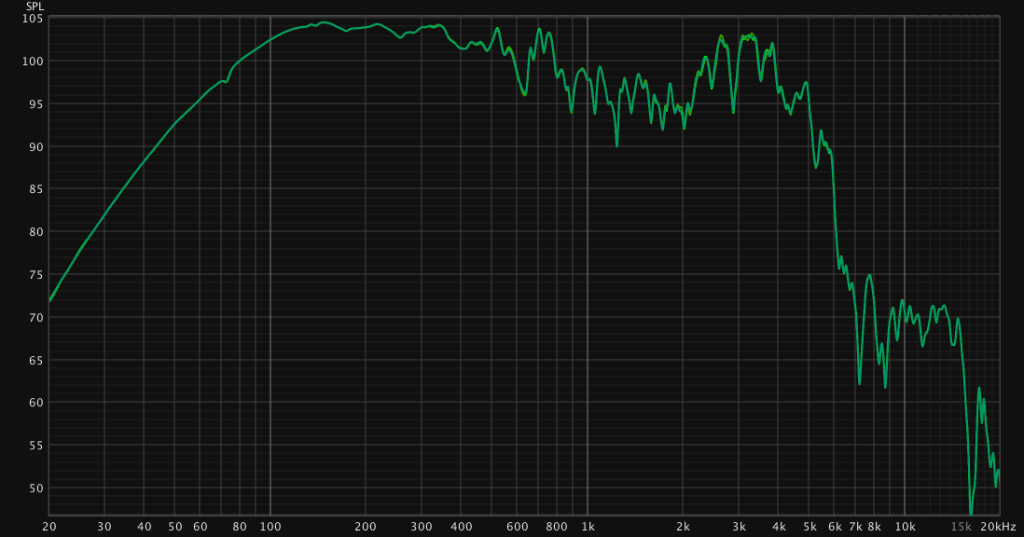
Let’s measure the THD of the guitar speaker under test:


The measurement shows that the THD reaches about 3% for most of the frequency range. Below 50Hz the distortion rises to close to 10%. I would consider everything below 50Hz out of band for a guitar signal. It seems like there is no fixed number at which the distortion becomes audible. The humans perception of non-linear distortion is not just dependend on the level but on spectral masking, time masking etc. As a rough guidance THD above 1-2% is audible. As a subjective hint – while measuring I did notice the distortion of the sine sweep at low frequencies and around 1-2k. So the simulation of the speaker with an IR will most likely have some audible differences with clean low frequency signals as well as some differences in the midrange.
There is also linear distortion. These are changes of phase and amplitude – luckely an IR can reproduce linear distortion.
3. Validating the setup
We also need to consider the system we’re trying to recreate.

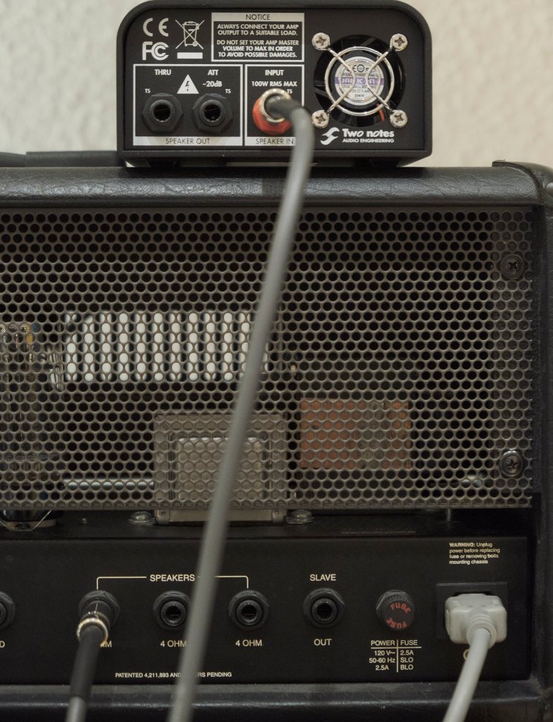
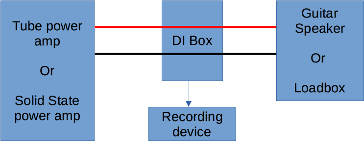
The real setup mirrors a recording setup with a real amp plus an out and loud guitar speaker recorded through a microphone. The simulated setup replaces the guitar speaker with a loadbox and guitar speaker IR. The setup can be simplified to a tube power amp into a loadbox with a guitar speaker IR applied to the signal. The reason the speaker needs to be split into the IR and loadbox components is, that a tube power amp interacts with the impedance of the speaker. This introduces linear and non-linear effects. To accurately recreate this effect the loadbox presents the same or similar impedance curve to the tube amplifier. It would also be possible to skip the power amplifiert all together and just record the preamp. Since tube amplifiers feature power amp tone shaping controls as well as power amp distortion which is important for some sounds I find it worthwhile to also use the tube power amp.
3.1 Loadbox validation
The loadbox used is the torpedo captor 8 Ohm. Let’s test if the loadbox sufficiently model the speaker. To test this the frequency response of the tube power amplifier was measured at the circuit level. This doesn’t include any acoustic factors – just the frequency response on the circuit level. The presence circuit of the tube amplifer was turned to zero and the vintage mode was used.
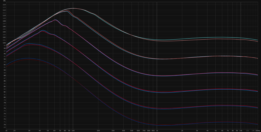
4 Setups were tested:
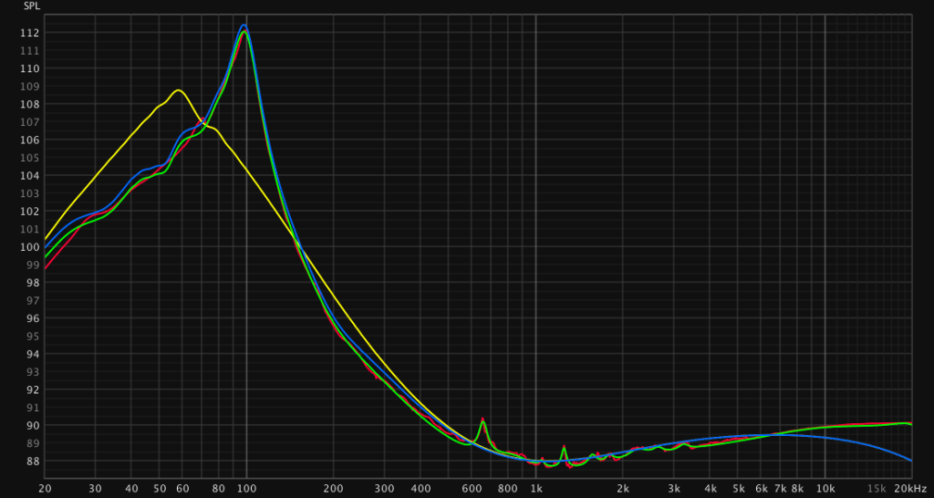
1. Mesa Boogie Single Rectifier Power Amp + Mesa Boogie 2×12 Vertical with V30s – red
2. Mesa Boogie Single Rectifier Power Amp + Loadbox – yellow
3. Solid state amplifier + Mesa Boogie 2×12 Vertical with V30s – green
4. Solid state amplifier + Loadbox – blue
Setup 1 is the real interaction between tube power amp and speaker. Setup 2 tries to imitate setup 1 and fails only in the bass region where the resonance of the speaker has a much higher peak at 100Hz while the load box peak is lower at 60Hz. There is some difference in the mids between 150Hz to 500 Hz which may sound “boxy” in comparison. There are slight variations in the 600Hz-3,5kHz range which the loadbox doesn’t reproduce. Also the loadbox tends to roll of the highs after 7kHz.
Setup 3 and 4 are basically the same. We can observe the high end rolloff of the loadbox is present as well. This means also we do not get any error when creating the impulse response from the interaction with the solid state power amp and speaker.
The loadbox produces a different power amp response curve than the 2×12 V30 speakers. Is this maybe intentional? Impedance varies with speaker type and wiring of the cabinet. Lets simulate a 1×12, 2×12 and 4×12 wiring of the same speaker. Unfortunately Celestion doesn’t publish the impedance curve of the V30 and I couldn’t find any third party measurements. But eminence manufactures the DV-77 which is based on the V30 and publishes the necessary data. So this comparison may not be entirely accurate but could give an indication why the load box impedance curve doesn’t match.
The DV-77 has only an 8 Ohm variant and the V30 used in the 2×12 are 12 Ohm. The simulation wires a 8 Ohm resistor in Series to essentially approximate the circuit of the 2×12 speaker cabinet. Most 2×12 V30 cabinets use the 16 Ohm Variant while 4×12 cabinets use the 8 Ohm variant to achieve 8 Ohm nominal when using a series-parallel wiring.
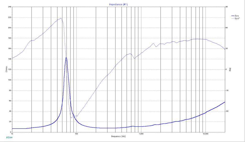
Basically the impedance is the same when cabinets are wired in the described way. (look up series and parallel resistance calculation 😀 )
This means two notes has either modeled a different speaker or wanted to create something different instead of a strict replication. To my taste the low end is cleaner and more defined with the loadbox. Probably because the peak is flatter. It could be that other tube power amp designs exhibit a different curve and the differences are not that large.
In any case to be more accurate we can derive a compensation EQ curve by matching the curves.
This is the filter set I derived using REW:
| Nr. | Type | Frequency | Gain | Q |
| 1 | bell | 33.70 | -1.8 | 2 |
| 2 | bell | 53.7 | -3.5 | 2 |
| 3 | bell | 99.3 | 9 | 2.81 |
| 4 | bell | 197.5 | -1.4 | 1.329 |
| 5 | bell | 659 | 1.8 | 11 |
| 6 | bell | 830 | 0.7 | 2.5 |
| 7 | bell | 1050 | 0.3 | 20 |
| 8 | bell | 1254 | 1.1 | 20 |
| 9 | bell | 1572 | 0.6 | 12 |
| 10 | bell | 1800 | 0.4 | 12 |
| 11 | bell | 2250 | 0.5 | 5 |
| 12 | bell | 2650 | 0.3 | 10 |
| 13 | bell | 3250 | 0.3 | 10 |
| 14 | High shelf | 7000 | 1.1 | |
| 15 | bell | 20000 | 1.5 | 0.500 |
While this filter set is rather complex to be done with a simple eq plugin I derived a simpler version with less bands which can be applied in a pinch.
| Nr. | Type | Frequency | Gain | Q |
| 1 | bell | 33.40 | -1.9 | 2 |
| 2 | bell | 53.7 | -3.6 | 2.003 |
| 3 | bell | 99.2 | 8.8 | 2.864 |
| 4 | bell | 200 | -1.6 | 1.466 |
Lets see how effective the filters perform on the load box frequency response.
The optimized EQ closely matched the original setup. There is some ripple in the response below 80 Hz but the ripple is less than 1dB. The simplified filter set is close enough. It misses a few peaks in the midrange and doesn’t compensate the falloff on the highs. This maybe irrelevant as the peaks are low in gain and have a small Q. The falloff in the highs reaches a -1-2dB at 10kHz which is not an important frequency range of the instrument and maybe even desirable. I shall later construct some listing tests to find out if the simple filter set is enough to practically compensate for the loadbox difference. For the purpose of matching the real setup with the loadbox setup I will use the optimized filters, unless stated otherwise.
I had a hunch – so I wanted to test of the differences of the power amp behavior between the speaker and loadbox are level dependent.
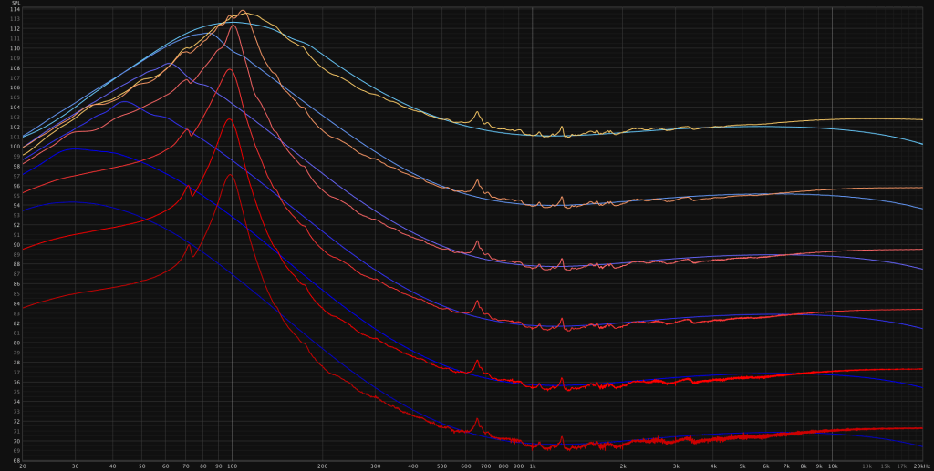
The difference between the load box and speaker interaction with the power amp seems to be level dependent. The lines in yellow/light blue color cast reach the limit of the power amp to amplify low frequencies. The resonant peak is clipped and the Q seems to be lowered. Lets just look at the behavior before the power amp starts clipping.
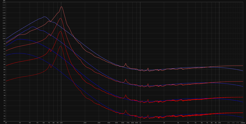
The power amp combined with the speaker behaves almost linearly with increasing level. Only the orange line exhibits a slight shift of the resonance frequency and not so linear scaling of the frequencies around 20Hz (insignificant).
The load box combined with the power amp does behave linearly except for the frequencies below 90Hz. Here we see a compression effect that scales with level and conversely with frequency. This is likely due to the load box having an impedance curve that probably looks like the dark blue curve.
The increased resistance might lead to a boost at lower frequencies until the power amp cannot deliver enough power due to the filter capacitors of the power delivery circuit not holding enough charge. The filter capacitors of this amp are, at the time of testing, about 20 years old. They may have degraded over time. This effect applies to any tube amplifier that reaches it’s limits. Increasing the filter capacitors beyond the original design would result in more thermal stress to the power delivery transformer(and output transformer) putting the amplifier at risk of thermal failure. – Not a viable option.
All electrolytic capacitors in the tube power amp have been replaced with the same values. The overall behavior didn’t change and the small difference can be attributed to the measurements being not exactly level matched.(The measurements were taken after servicing the amp)
To summarize the loadbox validation:
A corrective EQ can be applied to match the frequency response difference between the loadbox and the speaker for all frequencies above 100Hz. Below 100Hz the differences are non-linear and can be corrected to some extend but a 100% match cannot be achieved. The results are specific to this loadbox. Other brands may have smaller differences.
3.2 IR validation
Since we established, that the solid state power amp behaves linearly we can use it to just validate the speaker against the IR. Let’s look at pink noise and a dirac impulse recorded through the speaker and applied IR.

Well it definately doesn’t null. There is definatly a difference between the IR and the recording – especially in the high frequencies. But listening the files soloed I cannot hear the difference that is shown on the nulltest. The difference doesn’t seem to be rooted in the frequency response since listening test with noise reveal those easily. Lets try a guitar chord. Maybe with realistic programm material can reveal the difference.
It doesn’t null again – no surprise. But the differences are much more audible, though still slight. I percieve the microphone version to have slightly more upper midrange. And difference of the nulltest indicates that there is a difference in that region. So it is slightly audible. I think the difference is attributable to the THD of the loudspeaker, looking at the THD graph from earlier. Since the difference is so small for a realistic scenario it doesn’t matter.
3.3 IR + Loadbox validation
How close can we get when using an IR and loadbox instead of a real speaker. Test this a test signal will be run through the simulated setup and the real setup. Instead of a guitar signal a recording of the guitar preamp will be replayed through the FX loop to have a more consistant test signal. The test signal is a highly distorted guitar and the clean guitar chord from ealier. The distorted signal with a dense frequency spektrum will reveal the differences in frequency response while the clean signal will reveal the non-linear factors.
4. Optimizing IR parameters
First let’s list all of the parameters that come to mind:
- Method(sine sweep, dirac impulse etc.)
- Deconvolution program/reversed method
- Sweep length
- Sweep repititions
- Minimum phase or linear phase
- Samplerate and bit depth
- IR length
- Convolution program
4.1.1 Method
There are two popular methods of creating an impulse response. The Dirac impulse or the sine sweep method. The sine sweep method has the advantage that only one frequency has to be reproduced at a time so the system can be turned up louder but has the disadvantage that the signal was has to be deconvolved first. The sine sweep has a better SNR. Both methods support multiple passes and averaging to suppress noise.
Lets do the IR nulltest of the IR evaluation with the sine sweep and dirac impulse method.
Pink noise nulltest microphone recording vs sine sweep IR convolution
When listening to the pink noise files the dirac IR convolution has noticably less high frequency content while I cannot tell the difference to the sine sweep IR convolution. The nulltest shows the sine sweep has a larger difference in the midrange while the dirac version has major differences in the lows and highs.
Guitar signal convolved with dirac IR
Guitar signal convolved with sine sweep IR
Guitar signal nulltest microphone recording vs sine sweep IR convolution
When listening to the guitar signal test the differences are the same but less noticable.
Concluding the method comparison: I would choose the sine sweep method. The differences in my tests are to my ears inaudible. Also the SNR is higher that the dirac method.
4.1.2 Deconvolution Program
There are a multitude of programs that can record and deconvolve sine sweeps.
Notably I have used REW and Voxengo Deconvolver. The latter offers an interesting “reversed technique” which promises to reduce non-linear distortion.
https://www.voxengo.com/doc/deconvolver/
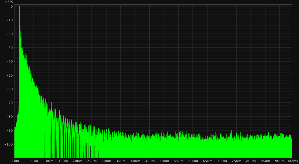
Well lets look at a comparison:
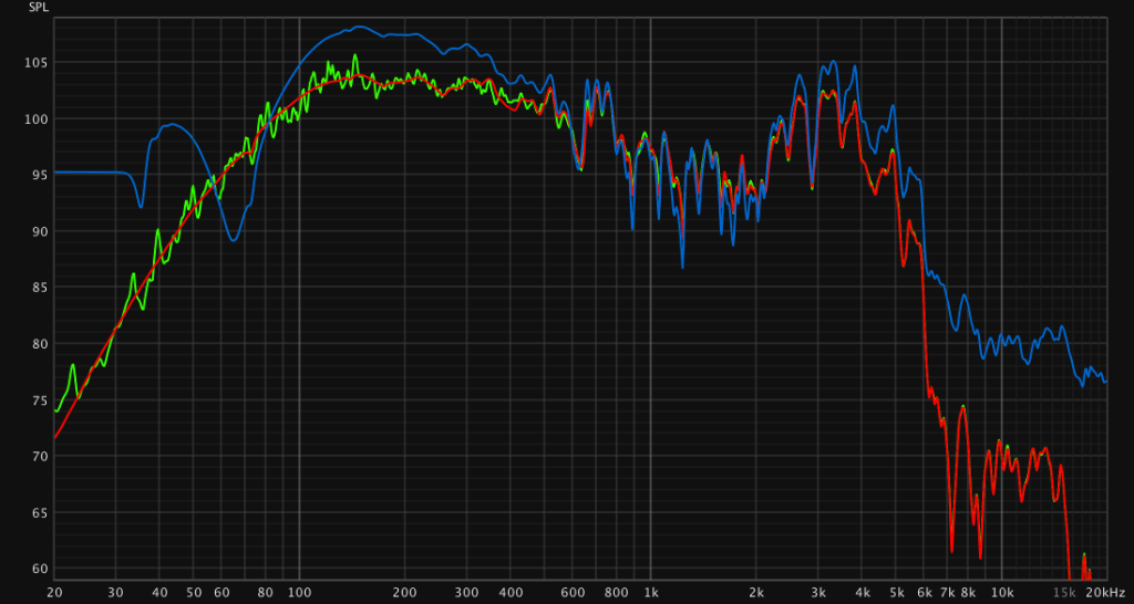
Blue: voxengo deconvolver reversed technique, red: REW sine sweep, green: white noise recording amplitude.
The reversed technique introduces significant errors at low and high frequencies. Thats sad – skip this function. But don’t necessarily skip voxengo deconvolver 😉
4.1.3 Sweep length
Lots of programs allow you to define the length of the sine sweep. However I could not find clear answers with a quick google research what is impacted by the length.

From light to dark: 2,7s, 5,5s, 21,8s, 80s
The frequency response doesn’t seem to be impacted by the sweep length. The sweep length could have had an impact by heating up the voice coil.
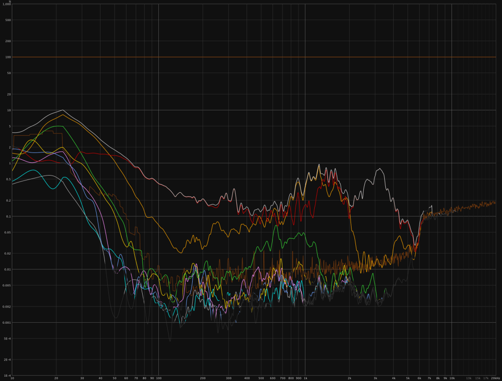

There seems to be no difference in noise and distortion performance when comparing the extremes (2,7s and 80s).

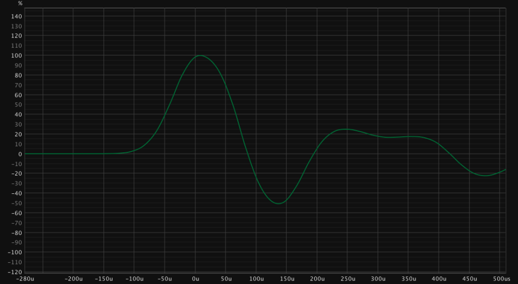
The initial transient seems to be basically identically execept for a deviation at 4,5ms.
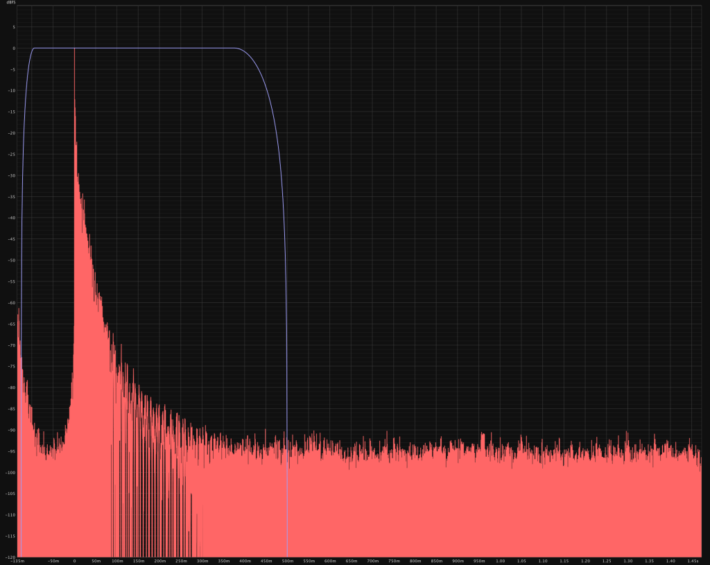

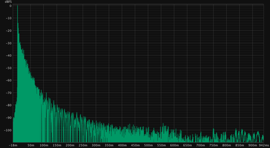
When looking at the noise floor of the impulse we can observe: that the longer the sweep, the lower the noise floor. At 2,7s length the noise peaks at -90dBFs while 80s length lower the noise to -108dBFs.
But how low of a noise floor is necessary?
We can answer that by looking at the necessary length of an IR and the signal level at that shouldn’t be covered by noise. Look at section 4.1.8 if you want the details why I decided that 500ms is a good target.
In an ideal world I would like the IRs to not introduce any perceptible noise. That would be below -120dBFs according to this post on audiosciencereview. Since the noise floor of the 80s measurement is still at -108dBFs it is simply not realistic when you want to measure a speaker for example 30 times. Different microphone combinations and mic placements will exceed that number easily. The looser limit that is mentioned in the post would be the 16bit noise floor of -96dBFs. This target is easier to hit and is more realistic, since a guitar rig rarily achieves 96dB of dynamic range anyway(nevermind distorted tones). In this case it took 5,5s sweep length to achieve this target.
To conclude the sweep length: Choose the sweep length so that a dynamic range from peak to noise of at least 96dB is achieved.
4.1.4 Sweep repetitions
A sweep can be executed multiple times and averaged to reduce noise in the measurement. This can only be done if the recording system is sufficiently synchronised and the measured system time invariant. Otherwise the avering will produce errors. I do not recomment averaging when combining input and output systems without clock sync like USB Microphones and a different DAC.
The frequency response is not affected if the system meets the requirements.
The noise floor is reduced. However the same can be achieved by playing a longer sweep. Only when a long continous sweep cannot be done because of thermal problem(usually tweeters etc) for example an averaging is recommended.
4.1.5 Minimum Phase vs. linear phase
When deconvolving the sine sweep recording many programs give the options to export a linear phase or minimum phase IRs.
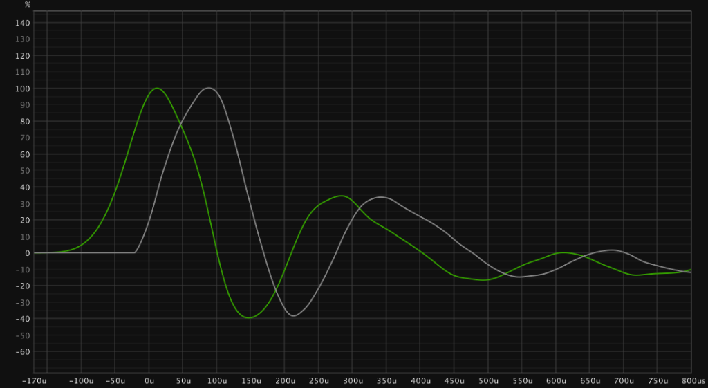
Basically the minimum phase version starts on a specific sample while the linear phase version has a less shallow slope.
The Dirac Impulse also shows the behaviour of the linear phase version. It seems like the linear phase version is more accurate and should be used.
4.1.6 Samplerate and bit deph
Because the SNR target of 96dB 24bit recording or better must be used. Yes, averaging could be done to circumvent sampling noise, but every professional recording interface can record 24bit – so do it!
The question of samplerate is not that easy and depends on the usecase.
Modelers like the line 6 or fractal products work at 48kHz and will convert any IR to the native samplerate. When working for audio for moving picture the sample rate is set to 48kHz as well. Only when working with CD a samplerate of 44,1kHz is required or when working for some streaming services higher samplerates can be used for the project. Highly distorted guitar tones can produce frequency content above 20kHz. But the perceptibility of frequencies above 20kHz is questionable at best. It depends on your measurement setup. Make loopback measurement and see if your equipment benefits from a higher samplerate.

The filter of this recording interface at 48kHz is adequate and higher samplerates could improve the measurement by 0,4dB at 20kHz. I do not consider this a reasonable improvement. If you need 44,1kHz use high precision SRC like the apple bats algorithm or the SRC that comes with your DAW. Or have twice the work when capturing – your choise.
To conclude samplerate and bit depth: 24bit with 48kHz. – UNLESSS your interface LPF sucks – then try 88,2/96kHz.
4.1.7 IR length and convolution program
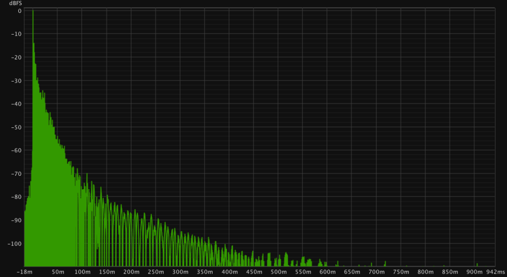
The IR length dictates two aspects: frequency resolution of the FIR filter and time information. Information after the IR has ended is lost. Meaning, if there are any events like room reflections or woofer resonance they can only be captured and reproduced when the length is sufficient to cover the event. I will not cover room reflections since they highly depend on the room. But the woofer resonance will be similar across guitar speakers.
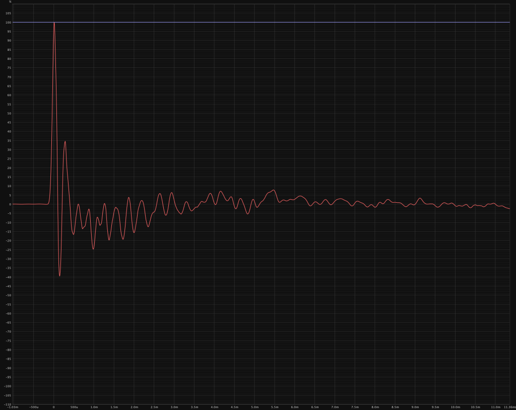
Let’s look at the woofer resonance decay:
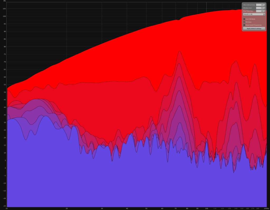
At 700ms the woofer resonance approaches the noise floor of the measurement. Obviously one could lower the noise floor by increasing the sweep length or averaging multiple sweeps but the resonance would decay indefinatly. In determining room characteristics we typically use the RT60 time which in this case would yield about 500ms RT60 for the woofer resonance.
“To get the optimum results the length should be 170 ms or more. The length of time you hold a chord is irrelevant. […] The impulse response of a speaker cab is typically much less than 100 ms. […] In my tests I’ve found that 8K samples (170 ms) is more than enough. I think 500 ms (24K samples) is overkill and if an IR has significant energy out that far then it has too much room in it.”
https://wiki.fractalaudio.com/wiki/index.php?title=Impulse_responses_(IR)
From the fractal audio wiki. It seems that 500ms is the usable limit of IR length. That is the case if you want to capture a dry IR without any long reverberations.
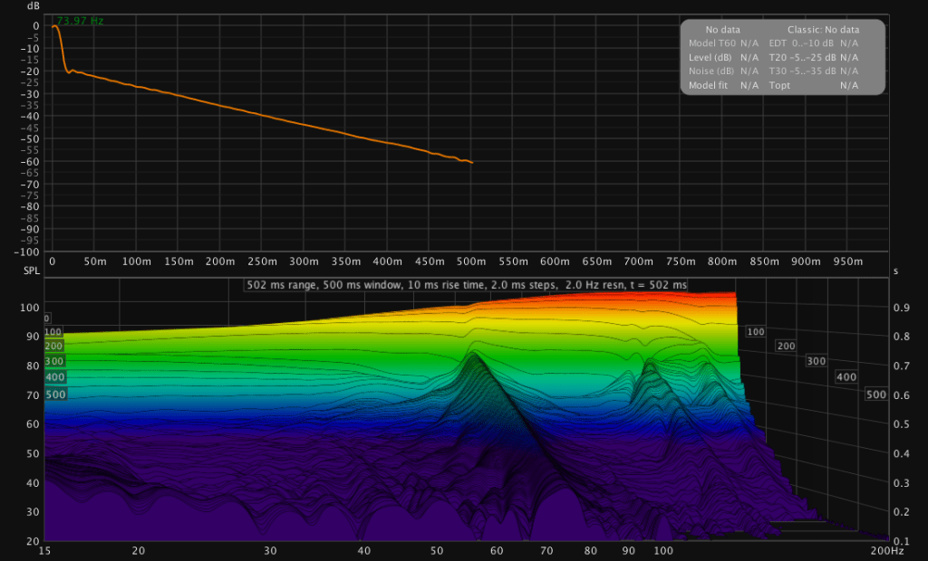
The second factor is frequency resolution. The resulting frequency resolution of a 500ms IR is 2Hz which is accurate enough to recreate the resonance of this speaker 73,5Hz with a Q of 36.75. That is more than enough.
The measurement shows the Q of the resonance to be about 24.5 which is a resolution of 3Hz. One would need 333ms to properly resproduce it. This is why 500ms is great because it leaves some headroom for narrower Q-factors. One should probably choose a length between 333ms-500ms.
Usually the IR will be longer. So you need to apply a window to the measurement. A rectangular window will introduce noise – especially when the signal level is still high (after 5-20ms for example).
“Normalization is your friend. Rectangular windows are simply truncation and are generally regarded as bad practice due to extremely high sidelobe levels. The choice of window is subjective. I actually use my own custom window that is not really a Hann window but that’s proprietary information.”
https://wiki.fractalaudio.com/wiki/index.php?title=Impulse_responses_(IR)
Basically it’s a tradeoff between frequency seperation(frequency resolution) and side lobe supression. Read more here. Since we increaded the IR length mainly because of frequency resolution I recommend the tukey window for the right side of long IRs since at the end of the IR the signal level will be low and the side lobes aren’t of interest. For the left side I would always recommend a very short tukey window to not introduce delay through the windowing function.
For shorter IRs <50ms I recommend a flat top or blackman-harris window on the right side to suppress noise since signal levels might still be high and a slight loss of frequency resolution is present because the IR is short.
To conclude IR length: between 333ms-500ms is fine for nearfield measurements. Use a very short tukey window on the left side. For long IRs use tukey on the right side. For short IRs use flat-top/blackman-harris.
4.1.8 Convolution program
The program that appplies the convolution is important. There are different kinds of programs:

Convolution Reverb
Convolution reverbs are most likely a plugin for a DAW. The maximum reverb length is either configurable or close to unlimited. Most convolution reverbs feature extensive controls and ways to apply further processing or change the IR. Convolution reverbs have the best quality at the cost of relativly high cpu usage and may have long processing latencies. Reaverb for example can be used in a zero latency mode (ZL checkbox).
Guitar IR loader plugins
Guitar IR loader plugins are basically limited convolution reverbs that additionally provide some functionality for mixing IRs. They typically limit the IR length to preserve cpu ressources. The quality settings influence the IR length:

Generally you want to pay attention to the length used and how the IR is windowed. In this case a rectangular windows is applied, newer versions might handle this differently.
DSP Hardware
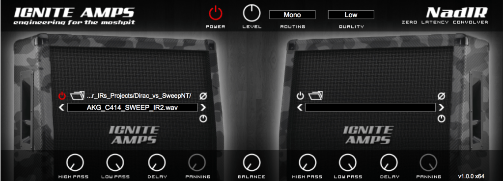
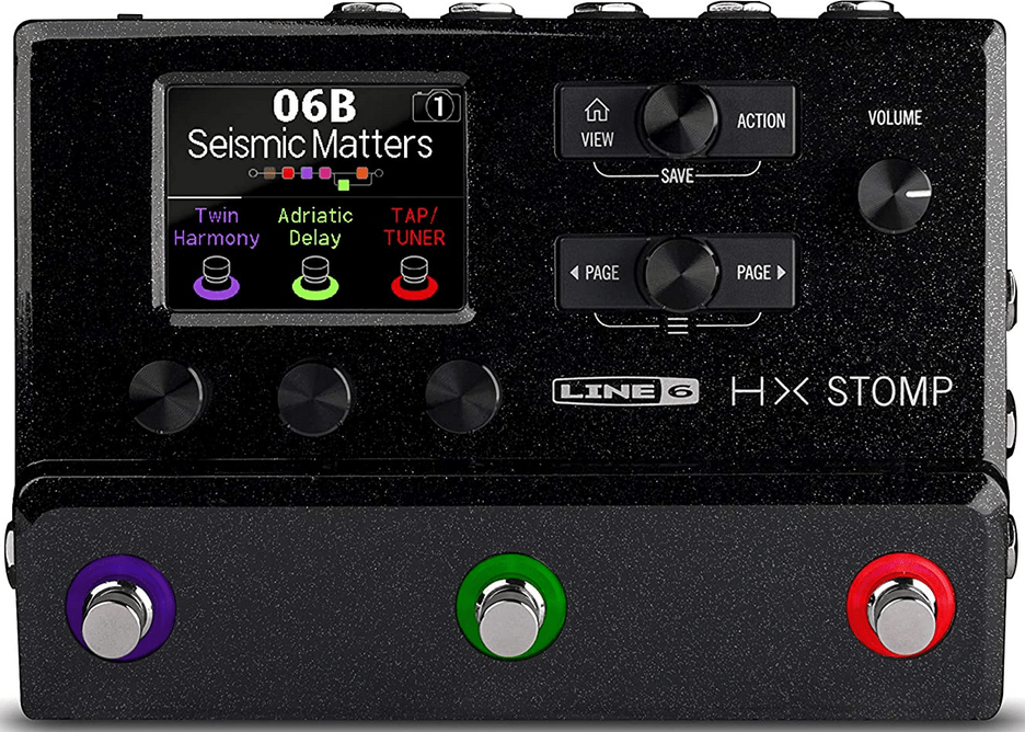
DSP hardware is everything from dedicated HW reverbs to guitar modelers with IR blocks. The features vary greatly as do the format the specific hardware does accept. The IR is length is most likely limited to multiples of 1024 samples and import programs truncate and window the IRs when importing IRs into the hardware memory. Almost all modelers operate on 48kHz while hardware reverb units feature multiple sample rates.
Read my analysis of the IR block of the helix line of products if you want specific information.
To summarize:
For best quality use a convolution reverb with the maximum length. For a more practical and less accurate version use a guitar IR loader to use the IR in while playing guitar. Switch to the highest quality while deciding on tones or during mixdown. Consider using a convolution reverb when recording is done.
DSP hardware is tricky to summarize and the specifics are very much hardware depended. At this point all I can say: RTFM!
4.2 Summary
TL;DR
Method: sine sweep
reversed method: no
Sweep length: as long as is needed to achieve 96dB SNR.
Sweep repititions: One. Increase sweep length if noise performance is not sufficient.
Minimum phase or linear phase: linear phase.
Samplerate and bit depth: 24bit/48kHz, unless audio interface sucks.
IR length: 333-500ms.
Convolution program: Convolution reverb for maximum quality, otherwise use what fits the specific use case.
5. More things to come
Let me say this first: Hit me up if you want me to look at something more in detail. I like to learn more and learn your usecases.
This investigation has brought up interesting things. Loadboxes seem imperfect and one of the weakest links in the chain. I want to build a impedance device that corrects the impedance to curve to more match the speaker. Also I want to measure other loadboxed – maybe there are more accurate ones out there.
IR parameters can be summarized into the previous TL;DR list. I think the convolution program and DSP hardware is worth more investigation. How IRs are truncated and how to best truncate them yourself to utilise shorter IR lengths or your DSP hardware as best as possible? I will investigate the specifics of the IR block and import process of the line 6 helix line since I own the device.
The whole world of mic placements and acoustic factors that might produce more subjective differences than technical answers is still to be explored. I’m interested to do a writup on that as well.
I will share some IRs as soon as I get to it. For now here are some examples I produced during testing:
GL;HF

Leave a reply to IRs from the Mesa 2×12 – Alpha Sonic Studio Cancel reply